Latin Hypercube Sampling
Introduction
Latin hypercube sampling (LHS) is a form of stratified sampling that can be applied to multiple variables. The method commonly used to reduce the number or runs necessary for a Monte Carlo simulation to achieve a reasonably accurate random distribution. LHS can be incorporated into an existing Monte Carlo model fairly easily, and work with variables following any analytical probability distribution.
Monte-Carlo simulations provide statistical answers to problems by performing many calculations with randomized variables, and analyzing the trends in the output data. There are many resources available describing Monte-Carlo (history, examples, software).
The concept behind LHS is not overly complex. Variables are sampled using a even sampling method, and then randomly combined sets of those variables are used for one calculation of the target function.
The sampling algorithm ensures that the distribution function is sampled evenly, but still with the same probability trend. Figure 1 and figure 2 demonstrate the difference between a pure random sampling and a stratified sampling of a log-normal distribution. (These figures were generated using different versions of the same software. Differences within the plot, such as the left axis label and the black lines, are due to ongoing development of the software application and are not related to the issue being demonstrated.)
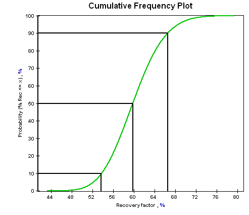
Figure 1. A cumulative frequency plot of “recovery factor”, which was log-normally distributed with a mean of 60% and a standard deviation of 5%. 500 samples were taken using the stratified sampling method described here, which generated a very smooth curve.
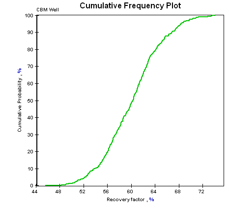
Figure 2. A cumulative frequency plot of “recovery factor”, which was log-normally distributed with a mean of 60% and a standard deviation of 5%. 500 random samples were taken.
Process
Sampling
To perform the stratified sampling, the cumulative probability (100%) is divided into segments, one for each iteration of the Monte Carlo simulation. A probability is randomly picked within each segment using a uniform distribution, and then mapped to the correct representative value in of the variable’s actual distribution.
A simulation with 500 iterations would split the probability into 500 segments, each representing 0.2% of the total distribution. For the first segment, a number would be chosen between 0.0% and 0.2%. For the second segment, a number would be chosen between 0.2% and 0.4%. This number would be used to calculate the actual variable value based upon its distribution.
P(X <= x) = n is solved for x, where n is the random point in the segment. How this is done is different for every distribution, but it’s generally just a matter of reversing the process of the probability function.
Grouping
Once each variable has been sampled using this method, a random grouping of variables is selected for each Monte Carlo calculation. Independant uniform selection is done on each of the variable’s generated values. Each value must only be used once.
Example
Average Joe has been offered free wood scraps from the local lumber yard. They tend to cut pieces up for customers and always have leftovers that nobody is interested in because the ends are damaged, or other contrived reasons. Joe wants to build U shaped picture frames out of these pieces, and he’s interested in knowing how probable it is that he can build a picture frame big enough for some strange purpose.
Joe’s odd U shaped picture frames require three pieces of wood. A base, and two sides. He’s going to make the base out of a chunk of 2-by-4, and the sides out of baseboards. The 2-by-4 (our first variable) comes in pieces 4cm to 40cm long, and the baseboards come in pieces 2cm to 60cm long. All possibilities are equally likely (uniform distribution).
We’re going to run this simulation with 10 iterations. (A common practice for Monte Carlo simulations is to start with about a thousand iterations, and work upwards depending upon the complexity of the problem.) We’re also going to use Python to do our simulation.
Sampling:
from __future__ import division
import random
iterations = 10
segmentSize = 1 / iterations
for i in range(iterations):
    segmentMin = i * segmentSize
    #segmentMax = (i+1) * segmentSize
    point = segmentMin + (random.random() * segmentSize)
    pointValue = (point * (variableMax - variableMin)) + variableMin
For our 2-by-4s, this might provide values like this:
| Sample | Segment Min | Segment Max | Segment Point | Value |
|---|---|---|---|---|
| 0 | 0% | 10% | 2.132 % | 4.767 |
| 1 | 10% | 20% | 13.837 % | 8.981 |
| 2 | 20% | 30% | 24.227 % | 12.722 |
| 3 | 30% | 40% | 33.716 % | 16.137 |
| 4 | 40% | 50% | 47.659 % | 21.157 |
| 5 | 50% | 60% | 53.636 % | 23.308 |
| 6 | 60% | 70% | 69.006 % | 28.842 |
| 7 | 70% | 80% | 73.106 % | 30.318 |
| 8 | 80% | 90% | 88.888 % | 35.999 |
| 9 | 90% | 100% | 90.812 % | 36.692 |
Once Joe has all three runs of the sampling for each variable, he’ll have a set of output like this:
| Sample | Variable 1 | Variable 2 | Variable 3 |
|---|---|---|---|
| 0 | 4.767 | 7.483 | 4.719 |
| 1 | 8.981 | 7.731 | 9.417 |
| 2 | 12.722 | 13.150 | 11.852 |
| 3 | 16.137 | 18.347 | 15.136 |
| 4 | 21.157 | 21.233 | 21.786 |
| 5 | 23.308 | 23.382 | 22.630 |
| 6 | 28.842 | 26.008 | 26.180 |
| 7 | 30.318 | 32.452 | 31.977 |
| 8 | 35.999 | 36.129 | 34.198 |
| 9 | 36.692 | 37.482 | 39.968 |
As you can see, even though both variable 2 and variable 3 have the same distribution (they’re the baseboards), the stratified sampling does not cause them to have the same numbers. It just causes a more evenly distributed set of numbers, eliminating the possibility of all 10 samples being the exact same number. In Monte Carlo simulation, we want the entire distribution to be used evenly. We usually use a large number of samples to reduce actual randomness, but the latin hypercube sampling permits us to get the ideal randomness without so much of a calculation.
The only step left is to shuffle these variables around to create some calculations. Joe’s software might randomly pick iteration 9 for variable 1, iteration 3 for variable 2, and iteration 5 for variable 3. This results in a set of (35.999, 13.150, 21.786) for the sizes of the 2-by-4s and the left and right baseboard. (Joe’s got a lopsized U! Not entirely unexpected. He should have been the guy buying the lumber first, the cheap bastard.)
Each number should be discarded after it is used, and others selected for the next calculation.
An alternative at this point is to run one case with each of the possible variable sets, creating 1000 calculations for these simple 10 variables. For complex cases involving many variables and many samplings, this can balloon to unreasonable numbers of calculations quickly. This eliminates all of the benefits that Monte Carlo simulation provides, while still providing approximately the same answer.
Conclusion
Latin hypercube sampling is capable of reducing the number of runs necessary to stablize a Monte Carlo simulation by a huge factor. Some simulations may take up to 30% fewer calculations to create a smooth distribution of outputs. The process is quick, simple, and easy to implement. It helps ensure that the Monte Carlo simulation is run over the entire length of the variable distributions, taking even unlikely extremities into account as one would desire.